Loan default predicition

Notice: This project was originally developed as part of my coursework for the MIT Applied Data Science Program (ADSP) that I attended in early 2024. Since completing the course, I have revisited and expanded upon the original project, incorporating additional analysis and fine-tuning the models to enhance their performance. As a result, the project presented here differs from the version submitted during my MIT ADSP course, reflecting these ongoing improvements and refinements.

Problem Statement

Mortgage loans are a highly profitable revenue stream for financial institutions. During the pandemic, when interest rates were particularly low, profit margins on mortgage lending were notably higher than the historical average of 0.6%, reaching 1.57% in 2020 and 0.82% in 2021.¹ This profitability is further evidenced by the number of firms offering mortgages, even when it represents only a small portion of their overall revenue. For traditional banks like JPMorgan Chase, mortgage-related earnings constitute roughly 1% of the total² while for non-bank lenders like Rocket Companies, over 75% of earnings come from mortgage loan offerings.³ While direct revenue streams like loan origination fees, interest income or secondary market sales make loans attractive to lenders, there are also indirect ways of generating income from mortgage clients. From a lender’s perspective, a borrower is locked in until the loan is paid off which takes several years at minimum. This opens up opportunities for cross-selling, i.e. offering alternative products by leveraging the customer data obtained by the lender. For borrowers, it’s simply more convenient to purchase from an institution they already do business with.

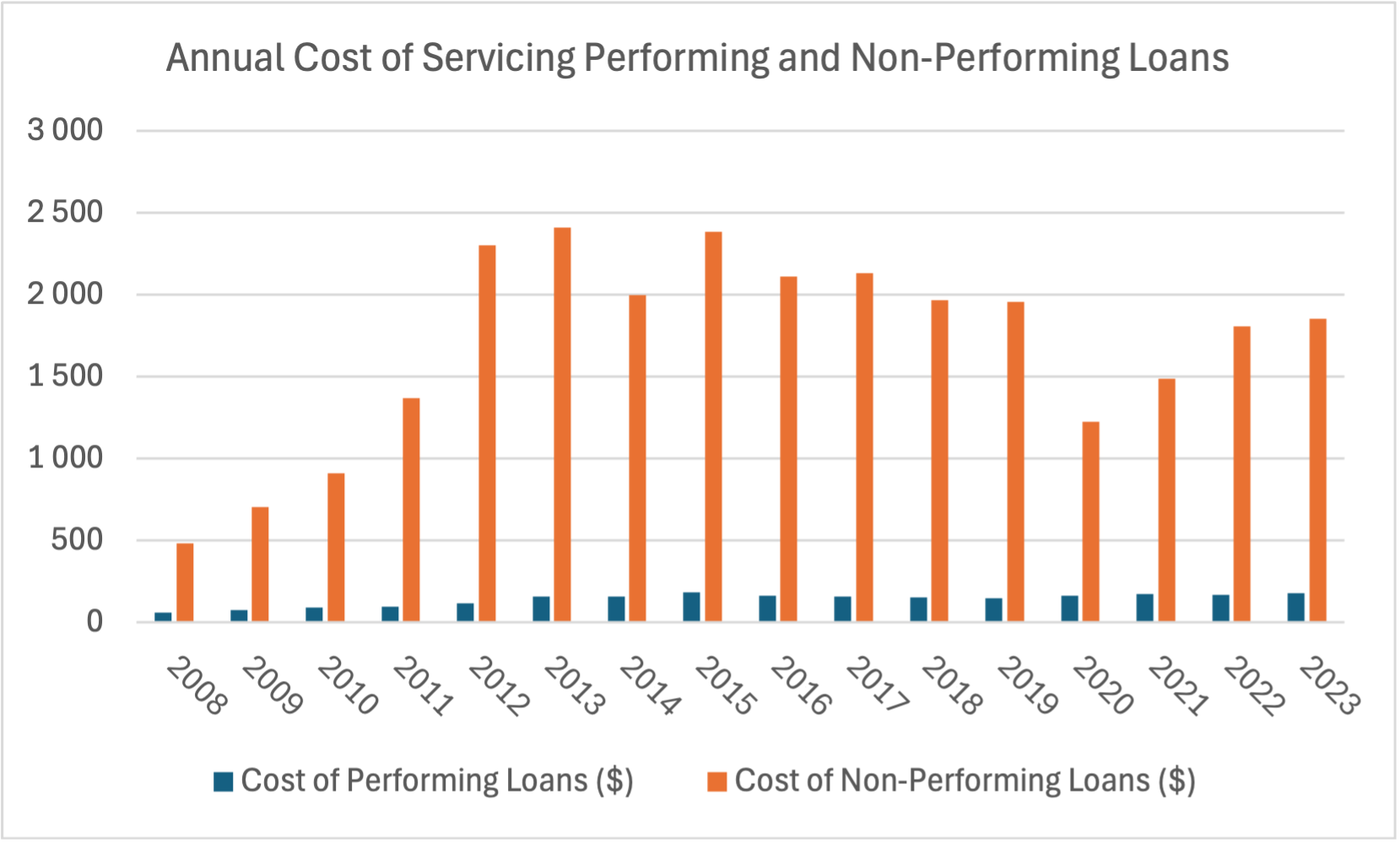
Conversely, home loans pose risks for lenders, the most significant being the risk of a loan defaulting when the borrower fails to make payments on time. Failure to collect loan payments requires the lender to classify the loan as a non-performing asset (or NPA). Carrying NPAs is detrimental to the banks cashflow, potentially signaling to the regulators that the bank’s financial stability is at risk. Furthermore, the average cost of servicing a non-performing loan in 2023 was over 10 times higher than a performing loan ($1,857 vs $176) as evidenced by Mortgage Bankers Association’s study on loan servicing. Therefore, it’s very important for the bank to mitigate the risk of loan default as early as possible by ensuring that the loans are issued only to customers who are able to pay them off in full.

Annual Cost of Servicing Performing and Non-Performing Loans — Source: MBA’s Annual Servicing Operations Study & Forum - www.mba.org/sosf

The objective of this project was to develop a tool to predict clients who are likely to default on their loan and give recommendations on the important features to consider while approving the loan. Additionally the model should be interpretable enough so that it is possible to provide the reasons for an approval or rejection of an application and adhere to the Equal Credit Opportunity Act’s guidelines⁴. Without getting into too much detail, the guidelines are meant to promote fairness and prevent discrimination in the credit industry, ensuring that all individuals have equal access to financial opportunities. The business stakeholder is the consumer credit department of a bank that wants to simplify the decision-making process for Home Equity Line of Credit (HELOC) loans. A HELOC loan provides a line of credit based on the equity in a home which is the difference between the market value of a home and the outstanding mortgage balance.

Data Description

The solution is based on data from recent applicants who have been given credit. The model should only use the data provided by the bank.

The dataset is a single csv file containing 13 features and 5960 observations of home equity lines of credit. The binary target variable BAD indicates whether the client defaulted on a loan (value of 1) or not (value of 0). The other 12 independent variables describe the financial, job and loan-specific situation of each client. For example REASON is the reason for the loan request (home improvement or debt consolidation), YOJ is the number of years at present job or CLNO is the number of existing credit lines. There are two categorical variables (of type object) and the remaining variables are numeric.

Exploratory Data Analysis (EDA)

Upon inspecting the data, I discovered numerous issues like missing values or outliers that needed to be addressed before proceeding with building the models. In this section, I explain how those issues were addressed and formulate observations about the patterns in the data that will be helpful in the model building phase.

Univariate analysis

Most of the variables were missing values and the volume of missing data varied from 2% to 21%.

Variable	% of missing values
`DEBTINC`	21%
`DEROG`	12%
`DELINQ`	10%
`MORTDUE`	9%
`YOJ`	9%
`NINQ`	9%
`JOB`	5%
`CLAGE`	5%
`REASON`	4%
`CLNO`	4%
`VALUE`	2%
`BAD`	0%
`LOAN`	0%

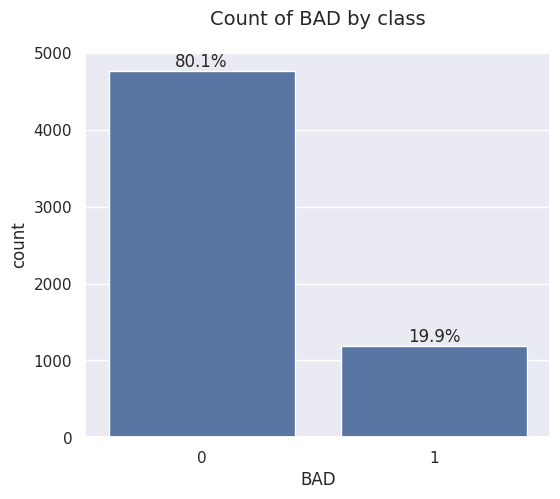
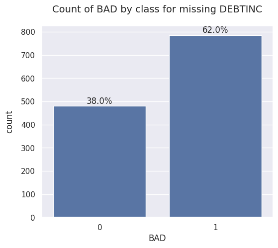
The missing values in the debt-to-income ratio variable DEBTINC were particularly troublesome because of the class imbalance in the target variable for observations where DEBTINC was missing versus the entire dataset. Looking at the entire dataset, there were 1189 (20%) instances where a client defaulted on a loan. Out of those, in almost 800 cases the applications were missing debt to income ratio information. Other variables with high number of missing values did not display a similar pattern of varying class imbalance.

Count of BAD by class — Target variable BAD distribution for all observations vs where DEBTINC is missing.

Count of BAD by class for missing DEBTINC — Target variable BAD distribution for all observations vs where DEBTINC is missing.

Upon analyzing the missing values, I identified two issues that needed to be resolved prior to the model building phase:

Issue #1: removing observations with missing values would significantly reduce the available dataset due to the volume of nulls and affect the class imbalance of the target variable. Therefore, missing values should be populated through imputation.

Issue #2: the example of DEBTINC showed the fact that an observation is missing is important to the outcome. Therefore, that information should be preserved in the model.

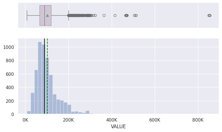
Several variables in the dataset were skewed to the right with majority of the data points concentrated around 0. This results in many outliers in the data that needed to be treated in order to avoid a situation where a model will not generalize well to the data. Observing the histograms and boxplots I noticed that continuous variables like LOAN, MORTDUE and VALUE had similar distributions with many outliers to the right.

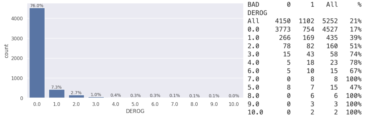
Boxplot and histogram of VALUE (current value of the property.)

For two discrete variables with few unique values — DEROG and DELINQ — all values outside of 0 were considered outliers because the majority of observations were 0. The charts below show the distribution of values for both DELINQ and DEROG, along with tables detailing the number of observations by the class of the target variable. All clients who had over 5 delinquent credit lines, and almost all clients with 7 or more derogatory reports, ended up defaulting on their loans.

Barplot for DEROG and distribution of BAD for each value of DEROG.

Barplot for DEROG and distribution of BAD for each value of DELINQ.

The findings above unveil another issue to be addressed:

Issue #3: several numeric variables contained some outliers. However, for variables DEROG and DELINQ all the values except 0 were outliers because of how many observations were actually 0. In those cases, all variance would have been lost after updating those observations. At the same time, the two features should not be excluded because, intuitively, both the number of derogatory reports and the number of delinquent credit lines are important factors indicating a person’s financial health. In fact, the number of late payments is a direct reason for flagging a loan as an NPA and potentially leading to default.

Multivariate analysis

First, I verified that the target variable classes were equally balanced for every value of the categorical variables JOB and REASON. Next, I investigated the correlation between the independent variables, and noticed there was a strong relationship between VALUE and MORTDUE.

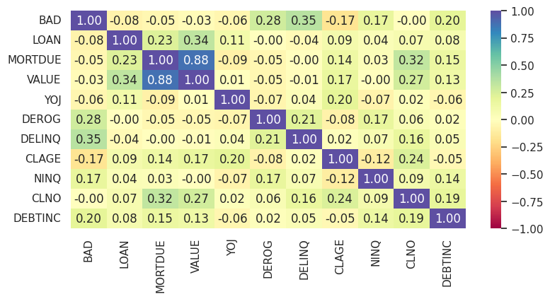
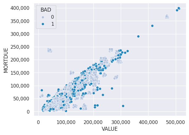
The correlation can be explained intuitively because the bigger the value of the property, the higher the mortgage usually is, although the two values are likely to diverge the older the loan becomes and the lager the equity. The scatterplot below confirms the linear correlation between VALUE and MORTDUE. There were no evident clusters of either good or defaulted loans present although for expensive loans (over 300,000), the number of defaulted loans becomes higher.

Scatterplot of VALUE vs MORTDUE for approved and unapproved loans. — Scatterplot of VALUE vs MORTDUE for good and defaulted loans.

For models that assume non-collinearity (for example logistic regression) it’s only possible to include one of the variables while for models that do not require that assumption (e.g. decision trees) both variables can be used.

Data preprocessing

In order to address the issues identified during EDA and to prepare the data for modelling, the following steps were applied:

Missing values for both numerical and categorical variables were filled in with median and mode respectively, which addressed issue #1 mentioned above.

New binary features with a _missing_values_flag suffix were created to indicate the missing values for each of the affected variables, which addressed issue #2.

Outliers were treated for all numerical variables except DEROG and DELINQ (due to issue #3) by replacing them with values of either lower boxplot whisker (Q1 – 1.5*IQR) or upper boxplot whisker (Q3 + 1.5*IQR).

Categorical variables were replaced with dummy variables using one-hot encoding.

For certain models that require scaling I applied a standardization algorithm using the StandardScaler function rescaling the features to have a mean of 0 and standard deviation of 1.

Modeling

Multiple models applicable to a binary classification problem were evaluated. The selected models were: Logistic Regression, k-Nearest Neighbors, Linear Discriminant Analysis, Decision Tree, Random Forest and XGBoost.

The data was split into a training and test set using a 70/30 ratio. Since the target variable classes were imbalanced, proportional weights were applied while training the models to counter theimbalance.

To score each model I used confusion matrices and associated metrics like precision, recall and F1 score. After analyzing all the models, I selected the primary metric for the final solution selection.

Logistic Regression

For the purpose of building a logistic regression model, the MORTDUE variable was excluded since it was strongly correlated with VALUE. The results showed consistent scores between training and test dataset with an F1 score of 0.69 and 0.71 respectively. To improve the results, I found a threshold that maximizes the F1 score on the training dataset. The precision and recall values to calculate the F1 score were obtained using the precision_recall_curve function from scikit-learn. The maximum F1 score of 0.73 was achieved at a threshold of 0.38. Applying that threshold to the test dataset, there was alo an improvement, albeit a slight one up to 0.72.

--- Training dataset ---
F1 score given .5 threshold: 0.69
Max F1 score: 0.73
Max F1 score threshold: 0.38
--- Test dataset ---
F1 score given .5 threshold: 0.71
F1 score for .38 threshold: 0.72

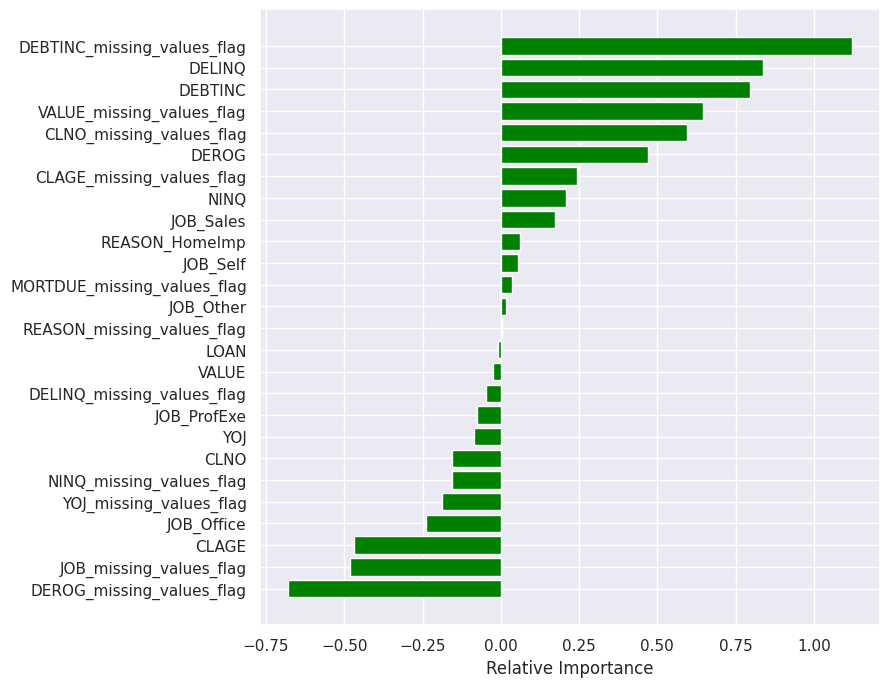
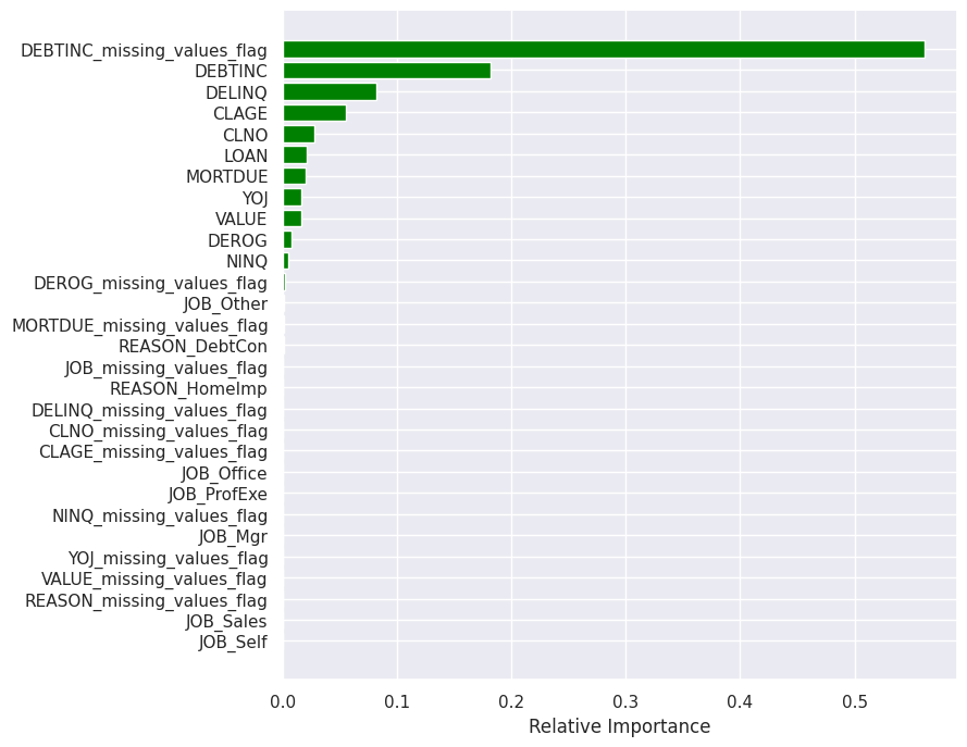
I also looked at the feature importance for the logistic regression mode to get an idea which variables are most important in making the classification decision. The most important feature was the missing debt-to-income ratio flag, followed by the number of delinquent credit lines and the value of debt-to-income ratio. Those three variables had a positive effect on the prediciton, meaning that the higher their value the bigger the probability of a client defaulting on a loan. Interestingly, a missing number of derogatory reports has a negative effect on the prediction.

Feature importance for linear regression.

k-Nearest Neighbors (kNN)

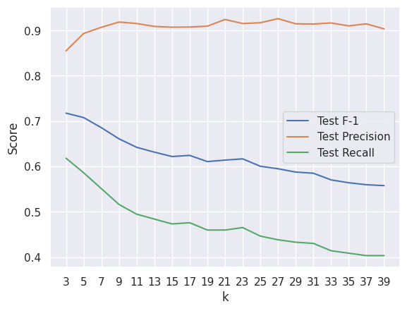
Since kNN is a distance-based algorithm and thus sensitive to scaling, I used the scaled features to train the model. To pick the optimal value of k (the number of nearest neighbors to consider), I ran the predictions and calculated the scores on the test dataset for a relatively wide range of ks (3 to 39). I only selected odd values of k to avoid ties in a binary classification problem. Leveraging the metrics functions from the scikit-learn library, I obtained precision, recall and F1 score for each k and visualized them on a plot.

As the number of nearest neighbors increases, the precision remains stable at around 0.9 while recall and, in consequence, F1 score gradually decrease. Therefore, I only considered low values of k in the model comparison stage. Similar scores were also observed on the training data, which means that the model is not prone to overfitting even for small ks.

Scores on the test dataset for different values of k.

Linear Discriminant Analysis (LDA)

Another algorithm I examined was LDA. Even though feature scaling is not necessary for LDA, I used the scaled features in this model because some of the variables like loan amount, number of derogatory reports and encoded categorical variables have significantly different scales. In order to fine-tune the hyperparameters I used a grid search algorithm. The customizable hyperparameters were solver and shrinkage. The n_components hyperparameter was not tunable because for binary predictions it’s fixed at 1. The solver parameter indicates the algorithm used to compute the solution and shrinkage applies the regularization intensity. Regardless of the optimization criteria (maximize F1 score, recall, precision) the best algorithm in each case was Singular Value Decomposition (SVD) where the shrinkage does not apply.

Best Parameters:
{'n_components': None, 'solver': 'svd'}

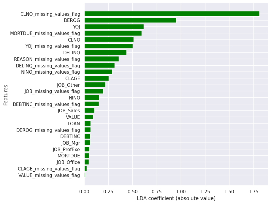
The LDA coefficients can be interpreted as a form of feature importance since the coefficients represent the linear combination of the features that best separates the classes. Larger absolute coefficient values suggest that a feature has higher influence on distinguishing between good and defaulting mortgages. Interestingly, the most important feature in the LDA model was missing number of credit lines (CLNO_missing_values_flag) which did not come up as one of the key features in most of the other examined models. Other impactful variables included number of derogatory reports, years at present job and missing amount due on existing mortgage.

Feature importance for the LDA model maximizing recall.

Decision Tree

For the purpose of building a decision tree model I included the MORTDUE variable that was excluded when building the logistic regression model due to colinearity. This decision tree gave a perfect 100% score on the training dataset. As for the test dataset the F1 score for class 1 was only 64% which meant overfitting. As a next step, I applied hyperparameter tuning to the decision tree using grid search in an effort to optimize performance. The hyperparameters tuned were criterion (gini, entropy or log-loss), the maximum depth of the tree (max_depth: 2-9), and the minimum number of samples at a leaf node (min_samples_leaf: 5,10,20,25). Depending on the maximized evaluation metric, the optimal hyperparameters were different as shown below:

Tuned hyperparameters for maximum recall:
DecisionTreeClassifier(class_weight={0: 0.2, 1: 0.8}, 
                      max_depth=5,
                      min_samples_leaf=25)

Tuned hyperparameters for maximum precision and F1 score:
DecisionTreeClassifier(class_weight={0: 0.2, 1: 0.8}, 
                      criterion='entropy',
                      max_depth=5, 
                      min_samples_leaf=10)

Note: For maximized recall, the optimal criterion function is gini. It does not appear in the parameter list because it is the default criterion for the DecisionTreeClassifier function. The hyperparameters have the same values when either precision or F1 score are maximized.

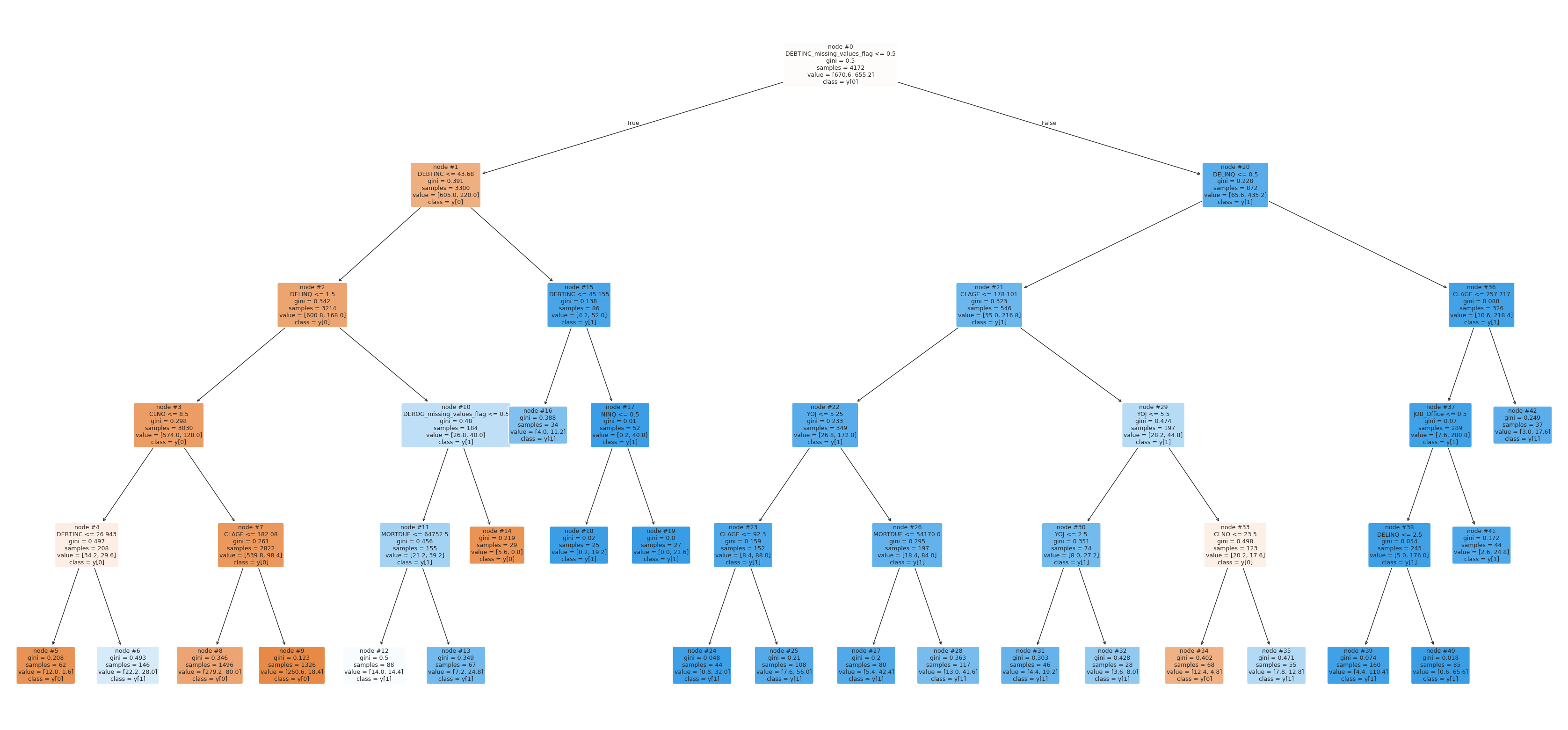
Maximizing recall yielded 84% on the training data and 80% on the test dataset. Precision was at 58% on the training and 54% on the test dataset. Maximizing precision yielded 64% on the training and 61% on the test dataset. The recall was at 79% on the traning and 77% on the test dataset. This means that the model does not overfit and generalizes well against the data. I plotted the decision tree to get an idea about the deciding features in the model and what might be the suggested business criteria for approving the loan application. For example, if the applicant has not provided their debt to income ratio and they have at least one delinquent credit line, then they should not be given a loan because they will likely default. On the other hand, if the applicant’s debt to income ratio is lower than 44, they have no more than one delinquent credit line and have at least 9 credit lines, they should be given a loan, regardless of other factors analyzed.

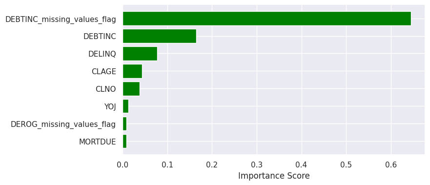
Decision tree diagram where recall is maximized.

Concurrently, the feature that was the most important in making predictions was DEBTINC_missing_values_flag, meaning that its inclusion resulted in the largest improvements to the purity of the splits. The second-most important feature was DEBTINC which was over three times less important than the missing debt-to-income ratio flag. The chart below shows eight most important features in the decision tree model.

Feature importance for the decision tree model maximizing recall.

Random Forest

Similarly to the decision tree model, I started with a basic classifier with weighted classes, fit it to the training data and evaluated the performance on the training and test dataset. The model gave a perfect 100% score on the training data and an 82% precision and 69% recall score on the test data which indicated overfitting. Even though the recall was lower compared to the decision tree, the precision improved. Next, I used grid search to find the hyperparameters that maximize precision, recall and F1 score. The tuned parameters were n_estimators (number of trees in the forest), max_depth (maximum depth of each tree), min_samples_split (minimum saples required to split an internal node), min_samples_leaf (minimum samples required to be at a leaf node), max_features (number of features selected randomly to be considered at each split), max_samples (number/fraction of samples to use for each tree) and class_weights. The optimal parameters are shown below.

Tuned hyperparameters for maximum recall:
RandomForestClassifier(class_weight='balanced', 
                      max_depth=9, max_features=0.9,
                      max_samples=0.8, min_samples_leaf=40,
                      min_samples_split=5, n_estimators=120)

Tuned hyperparameters for maximum precision and F1 score: 
RandomForestClassifier(class_weight={0: 0.2, 1: 0.8}, 
                      criterion='entropy', max_depth=8, 
                      max_features=0.9, max_samples=0.8,
                      min_samples_leaf=30, 
                      min_samples_split=5, n_estimators=120)

Note: Similarly to the decision tree model, the optimal criterion function is gini.

The final scores did not differ much between the two models. For the first one, the maximized recall was 78% on the traning data, while precision was 59% and F1 score was 67%. The F1 score was maximized at 68%, with precision at 61% and recall at 76% on the training data. Looking at the feature importance plot, only two features stand out compared to the rest: missing debt-to-income ratio flag and debt-to-income ratio. The relative feature importance for both models looks very similar with more importance given to DEBTINC_missing_values_flag in the model wit maximized recall.

Relative feature importance for the random forest model maximizing recall.

XGBoost

I started analyzing the XGBoost algorithm with a baseline model containing default parameters and a logloss evaluation metric. That model had a perfect 100% score on the training data and a 75%, 84% and 79% recall, precision and F1 score respectively. For fine-tuning the hyperparameters I again used grid search to evaluate models that maximize precision, recall and F1 score separately. The following parameters were subject to tuning: n_estimators (number of trees), learning_rate (shrinkage to prevent overfitting), max_depth and colsample_bytree (fraction of features to consider at each split). Regardless of the score maximization criterion, the optimized hyperparameters were the same.

Best parameters found:  
{
'colsample_bytree': 0.5, 'learning_rate': 0.2, 
'max_depth': 5, 'n_estimators': 150, 'subsample': 1.0
}

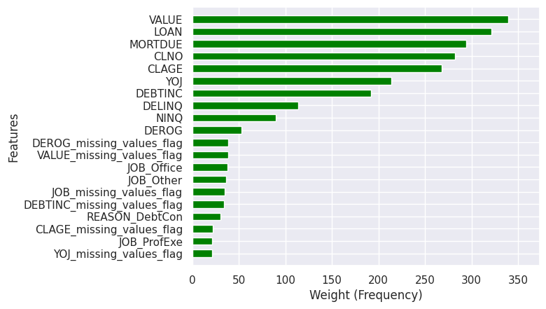
For that model setup, the performance metrics on the training data were as follows: 75% recall, 82% precision and 79% F1 score. I plotted a feature importance chart for the top 20 features based on the weight (frequency) measure which is the number of times a feature is used to split the data across all trees in the model. Notably, the most important features in decision tree, random forest and logistic regression are relatively less important in the XGBoost model. Specifically, in XGBoost all the missing values flag variables and categorical variables are less important than any of the numeric variables. The five most prominent variables are the loan amount, the value of the proprty, amount due on mortgage, number of credit lines and age of the oldest credit line.

Feature importance by weight (frequency) for the XGBoost model.

Results

In order to pick the correct evaluation metrics, I performed additional research to better understand the impact of mortgage defaults on the banks. Goodman (2016)⁵ points out that even though the percent of mortgages expected to go 90 days delinquent was at record lows in 2015, getting a mortgage was harder than earlier and banks were rejecting applications with even the slightest chance of default because of how much more expensive servicing a delinquent loan is in comparison to a performing loan. Since the bank wanted to avoid the risk of granting a loan to an individual who might eventually default, the goal was to minimize the number of false negatives. As a result, the primary metric used for model evaluation was recall. However, precision should also play a secondary role in the final solution design, in case the bank wishes to avoid losing potential clients by mistakenly flagging them as likely to default.

The table below displays each model’s accuracy, precision, recall, and F1 score for class 1 of the target variable on both the training and test datasets. The models are sorted by their highest recall scores. For the logistic regression model, the threshold was adjusted to 0.38 to achieve the maximum F1 score. For the decision tree, random forest, and XGBoost models, I evaluated both baseline and tuned versions, with the tuned versions optimized to maximize recall. For the LDA model, only one version was considered because its hyperparameters remained consistent regardless of the optimization criteria. For the kNN algorithm, I evaluated two options (k = 3 and k = 5), as these values yielded the highest recall and precision compared to higher values of k.

Model	Train F1 score	Test F1 score	Train precision	Test precision	Train recall	Test recall
Logistic Regression	0.644	0.652	0.514	0.536	0.859	0.831
Decision Tree tuned	0.684	0.647	0.577	0.542	0.839	0.803
Random Forest tuned	0.708	0.671	0.624	0.589	0.816	0.778
XGBoost tuned	0.976	0.786	0.996	0.822	0.957	0.751
XGBoost	0.999	0.793	1.000	0.842	0.998	0.749
Random Forest	1.000	0.753	1.000	0.799	1.000	0.711
LDA	0.690	0.709	0.716	0.774	0.665	0.653
kNN n=3	0.841	0.718	0.934	0.855	0.764	0.618
Decision Tree	1.000	0.638	1.000	0.661	1.000	0.616
kNN n=5	0.780	0.708	0.927	0.893	0.671	0.586

The model with the highest recall on the test dataset was logistic regression. Compared to other models, the recall scores between the training and testing datasets were similar which indicates that the logistic regression model does not overfit and generalized well to the data. Another benefit of logistic regression is that it is an interpretable model because the coefficients indicate how much each feature contributes to the classification result. Below are the most important features with their coefficients (greater than 0.5) and interpretation. The entire list of feature importances was presented on a plot in the modeling section.

Feature	Coeff.	Interpretation
`DEBTINC_missing_values_flag`	1.1	Applicants who do not provide a debt-to-income ratio are more likely to default on a loan and the odds of defaulting increase by a factor of 3. $e^{1.1}=3$
`DELINQ`	0.85	The more delinquent lines of credit the applicatn has, the higher the chance of defaulting. A one standard deviation increase of `DELINQ` increases the odds of defaulting by 2.34. $e^{0.85}=2.34$
`DEROG_missing_values_flag`	-0.67	Applicants with missing number of derogatory reports are less likely to default with odds of defaulting increasing by 51% for those individuals. While this might be counter-intuitive, it is possible that a missing value means zero derogatory reports but further investigation into the source data is required to verify this assumption. The number of derogatory reports variable (`DEROG`) indeed has a positive coefficient of 0.45. $e^{-0.67}=0.51$
`DEBTINC`	0.66	The higher the debt-to-income ratio, the greater chances of default. A one standard deviation increase of `DEBTINC` results in a 1.93 increase in odds of defaulting. $e^{0.66}=1.93$
`VALUE_missing_values_flag`	0.59	Clients with a missing amount on the application are more likely to default and their odds of defaulting increase by 1.8. $e^{0.59}=1.8$
`CLNO_missing_values_flag`	0.58	Clients with a missing number of existing credit lines are more likely to default and their odds of defaulting increase by 1.79 $e^{0.58}=1.79$

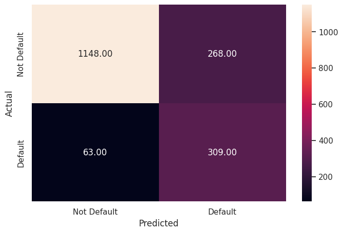
The downside of the logistic regression model was that the precision score was the lowest amongst all the models which means that applicants who would not default on a loan were relatively often flagged as likely to default, resulting in a loss of potential customer base. The confusion matrix for the test dataset illustrates that while the number of people who actually defaulted but the model failed to identify was low (63 out of 309 total defaults), the number of people who did not default but the model identified them as defaulting was relatively high (268) meaning that the model strict when it comes to evaluating applications.

Confusion matrix for the logistic regression model on test dataset.

Conclusion

On one hand the logistic regression model offers satisfactory results in terms of recall (83%) and it is easily interpretable. On the other hand, precision is low at 54% and the bank might lose potential revenue and reputation by not granting loans to financially well standing individuals. In order to mitigate that, the proposed final solution is a combination of two models, executed in parallel: logistic regression and XGBoost. XGBoost has one the highest precision scores at 84% but relatively lower recall compared to the logistic regression. Unfortunately, XGBoost is not as interpretable as logistic regression due to it being an ensemble model consisting of multiple trees. In an effort to identify key features, I created a chart in the modeling section where features were sorted based on the frequency measure which was a proxy for feature importance. This method however does not provide local interpretations (i.e. does not explain why a feature is important for a specific prediction) and it tends to be biased towards high-cardinality features (e.g. VALUE, LOAN) even if those are not truly important. It’s worth noting that kNN model had even higher precision numbers than XGBoost but much lower recall and lack of interpretability in terms of fearture importance because it does not learn parameters as a distance-based model. The dual-model approach ensures that there is a balance between recall and precision and provides an extra level of scrutiny in case the two models have differing predictions.

Recommendations

The final recommended solution consists of deploying two models – a logistic regression model and an XGBoost model. The logistic regression will act as a primary model and XGBoost will act as a secondary (support) model.

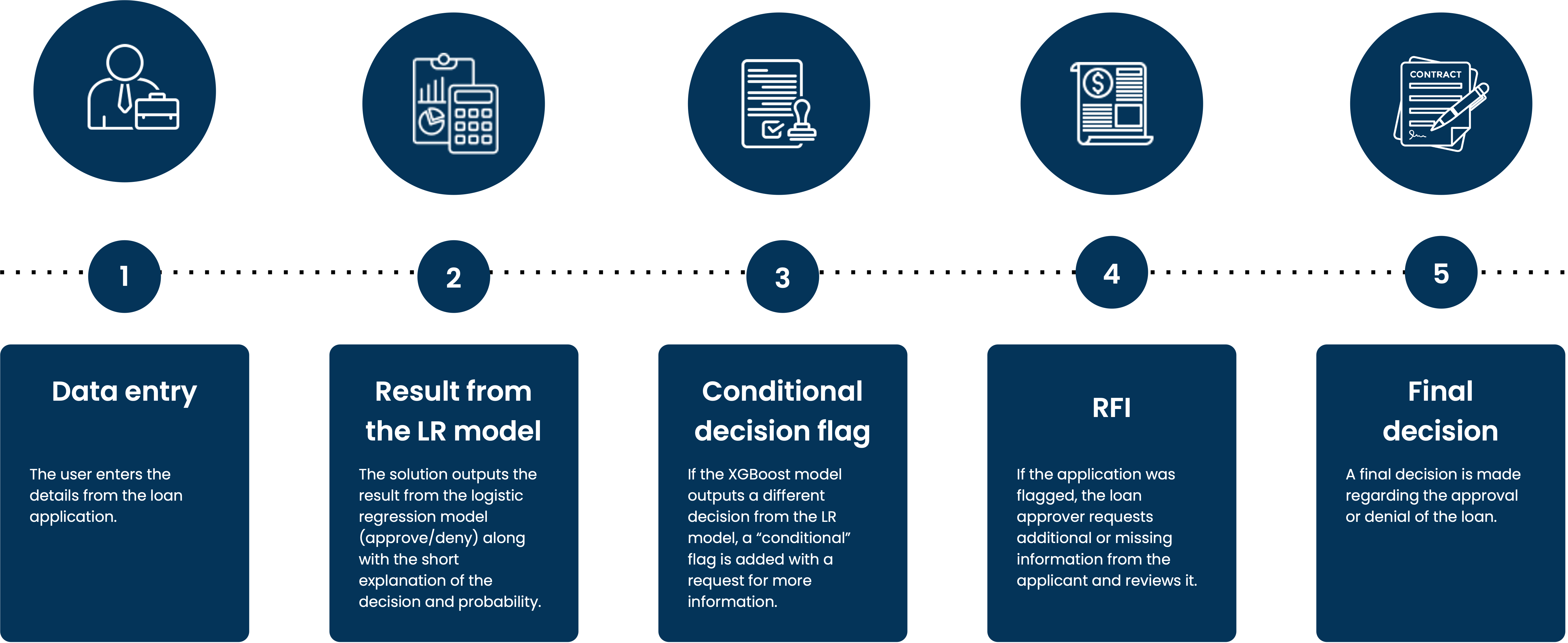
If, based on the input data, both models output the same result, the user will receive a decision recommendation (approve/deny) and a brief explanation of the features and values that led to the decision along with the resulting probability and threshold. If the models return different results, the user will receive a decision recommendation from the logistic regression model together with a “conditional” flag that will alert the user that more information will need to be provided in order to make the decision. Some examples of additional information might include tax and bank statements showing available assets or a questionnaire asking to provide data for any missing values.

There are several reasons for this approach. One is that it meets all the criteria set forth by the consumer credit department, i.e., interpretability of results (logistic regression), robustness (high recall of logistic regression combined with high precision of XGBoost) and highlights the most important features in the decision-making process. Another reason is the lack of relevant data. As Gamong and Noel (2020)⁶ conclude, only 3% of defaults are caused exclusively by negative equity. Most defaults are caused by features that the mortgage servicing data does not contain like current income or triggering life events such as job loss, divorce illness or injury. Moreover, Farrell, Bhagat and Zhao (2018)⁷ find that default rates for homeowners with small financial buffers were higher regardless of income level or payment burden. Asking clients to provide the above data points gives a more realistic view of their situation and it would show whether it is affecting loan repayment.

Providing exact numbers to quantify the benefit of the proposed solution is challenging. However, by taking the numbers from the provided dataset we can estimate the amount of money the bank would save by screening the applicants using the model solution. Assuming that the logistic regression model correctly identifies borrowers likely to default 83% of the time, the bank could have avoided servicing $90.8 million in defaulted loans if it were to use the proposed model ($\text{total value of defaulted loans} * 83%$).

A key challenge with the proposed solution is the fact that a model based on data collected at the time of mortgage application will not capture some key life events (job loss, illness, injury, catastrophe) or macroeconomic events (recessions) that might happen throughout the duration of the mortgage which might be several decades long. Historical mortgage delinquency rates (FRED 2024)⁸ indicate that economic events such as the subprime mortgage crisis or COVID-19 pandemic have an effect on mortgage delinquencies. To address these challenges, the bank and data science team should explore additional macroeconomic data sources like unemployment rate or inflation expectations. They should also consider financial and demographic data while keeping regulatory restrictions in mind. More research should be conducted to identify solutions that effectively model such occurrences, thereby enriching the proposed model. Some of the suggested approaches include time-series analysis like Vector Autoregression or scenario-based simulations using Bayesian Networks or Recommendation Systems.

Marcin Juchnowicz